To develop and validate the deep learning method for classification of crops using hyperspectral digital data

S. Jamalaiah^1* and K. Manjula Vani^{2 *}Correspondence: S. Jamalaiah, Department of Spatial Information Technology, Jawaharlal Nehru Technological University Hyderabad, UCEST, Kukatpally, Hyderabad, 500085, India, Email: ,

Author info »

Introduction

Images with a high spectral resolution are known as hyperspectral images. Which include more spectral data that can be used to understand and analyses spectrally comparable materials of interest [1]. Hyperspectral data were broadly used in land use land cover mapping, agricultural, mineralogy, physics, medical imaging, chemical imaging and environmental studies [2]. NASA's Jet Propulsion Laboratory (JPL) first proposed hyperspectral remote sensing in the early 1980s and it has since become an essential tool for remote sensing.

Crop identification and classification is an essential part of agricultural production. Crop classification and identification using hyperspectral remote sensing data is a difficult undertaking [2]. Classification and identification of crops using hyperspectral images are high dimensionality and spectrum mixing makes this a difficult undertaking [3].Barefaced computation and classification of the target and identification of crops imply more low accuracy and high cost of computation [3]. Usually, hyperspectral data suffer with limitation of available labeled training samples. Obtaining these samples is expensive and time consuming. A vast variety of classification methods to deal with hyperspectral data have been suggested in the time since the past decemvirate [4].

Because the scale issues, traditional classification algorithms (which can be divided into spectral-based and object-oriented methods) struggled to classify crops using hyperspectral data [5]. Support Vector Machine (SVM), K-Nearest Neighbor (KNN), Logistic Regression (LR), and Neural Network (NN) are examples of traditional classification approaches that focus on the usage of spectral features. Due to noise and other variables, the majority of these approaches result in low classification accuracy [6]. Many deep learning models have been used to classify and identify crops using hype spectral images in recent years. Stack auto encoder (SAE) [6], deep belief networks (DBN) [6], and CNN [7] are examples of classic deep learning models.

Materials and Methods

Related work

In recent past deep learning methods were very useful for the classification crops using hyperspectral data. Many methods for hyperspectral image classification have been proposed in the literature. Yan et al., [8], leveraging google street view images, suggested a deep leaning method for crop type mapping [8]. The authors used a Convolutional Neural Network (CNN) to classify the google street view images automatically. The overall accuracy for identifying normal images was reported to be 92% [9]. A hyperspectral image classification approach based on a 3D CNN model was proposed [9]. The authors of this article use 3D CNN and J-M distance to classify hyperspectral images. In both datasets, the total accuracy for classifying different crops was reported to be 92.50%. Bhosle et al., [2], CNN and convolutional auto encoder are two deep learning methods that have been suggested [2]. In this research, the authors used both methods to extract features before using PCA to reduce dimensionality. Both methods are 90% and 94% of the total accuracy, respectively. Ahmadi et al., [10], in this article on hyperspectral image classification; a Spectral-Spatial Feature Extraction (SEA-FE) approach was presented [10]. Spectral feature reduction using Minimum Noise Fraction (MNF) is used in this method to obtain pixel feature maps, which are then used to compute SEAF.

The hyperspectral image classification was found to have an overall accuracy of 92.13% [11]. For hyperspectral picture categorization, a multi-source deep learning method was proposed [11]. In this method, numerous hyperspectral images are used to train a model, which is then applied to the target hyperspectral image. A 98.8% overall accuracy was reported for classifying target hyperspectral images. Konduri et al., [12] proposed an approach to map a crop across the United States (USA) before harvest [12]. The first stage in crop classification in this approach was to build phenoregions using Multivariate Spatio-Temporal Clustering (MSTC). Based on spatial concordance between phenoregions and crop classes, the next step was to assign a crop label to each phenoregion.

Zhong et al., [13] presented a conditional random field classifier for a deep convolutional neural network [13]. Crop categorization using UAV-borne high spatial resolution images is presented in this framework. The overall accuracy of the WHU-Hi-Han Chuan dataset was 98.50% [13]. Through the integration of multi temporal and multi spectral remote sensing data, the Deep Crop Mapping (DCM) model was introduced, which is based on long short term memory structure with attention mechanism [14]. This method gets 95% accuracy for crop classification. Srivastava et al., [5], for pixel classification in hyperspectral images, deep CNN feature fusion, manifold learning, and regression are suggested [5]. The major goal of this project is to increase hyperspectral image categorization accuracy. This approach has a classification accuracy of 98.8%. Ji Zhao et al., [15] presented a conditional random fields-based spectral-spatial agricultural crop mapping method [15]. It uses the spatial interaction of pixels to improve classification accuracy by learning the sensitive spectral information of crops using a spectrally weighted kernel. Overall crop classification accuracy was 88.24%. Zhong et al., [16] provided a deep learning-based categorization framework for remotely observed time series data [16]. This method classifies the summer crops using the land sat Enhanced Vegetation Index (EVI) time series. In this method, they design two deep learning models; one is Long Short-Term Memory (LSTM), and the other one is one-dimensional convolutional layers (conv1D). The highest accuracy (85.4%) was achieved by the conv1D-based model [17]. Using Sentinel-1A time series data, three deep learning models for early crop classification were proposed [17]. One-Dimensional Convolutional Neural Networks (1D CNNs), Long-Short-Term Recurrent Neural Networks (LSTM RNNs), and Gated Recurrent Neural Networks (GRU NNs) are all used in deep learning models. For early crop classification, the most effective strategy combines all three models with an incremental classification method. This strategy offers a fresh look at early farmland mapping in overcast environments [18]. For crop categorization, a novel 3-Dimensional (3D) Convolutional Neural Network (CNN) has been proposed [18]. Images from spatio-temporal remote sensing are used in this strategy. Using spatiotemporal remote sensing pictures, crop categorization accuracy was 79.4%.

Area for study

This research area can be found in Ranga Reddy district, Telangana state, India (Longitude: 78.2752°E, Latitude: 17.5111°N), covering an area of 500 hectares. The climate of the study area is semi-arid. In this region, major crops are chickpea, groundnut pigeon pea, pearl millet, sorghum. These crops were harvested by the time the data was acquired. Figure 1 shows the study area map of ICRISAT.

Figure 1: Study area map.

Proposed methodology

To classify hyperspectral images, a customized 3D-CNN is used. This study focuses on preprocessing, image patching, and customizing 3D-CNNs to classify AVIRIS-NG hyperspectral data. The entire framework includes four stages:

1) Data Acquisition

2) Pre-processing

3) Image patching and splitting the samples

4) Apply neural network model.

The Figure 2 shows the entire framework.

Figure 2: Flowchart to develop and validate the deep learning method for classification of crops using hyper-spectral digital data.

Data acquisition

The Indian Pines dataset and the AVIRIS-NG data for the ICRISAT study area were used in this investigation.

Dataset of Indian pines: There are 220 spectral bands in the Indian pine dataset, with wavelengths ranging from 0.4 µm to 2.5 µm. This was obtained in 1992 at the Indian Pines test site in north-western Indiana, US, using Airborne Visible Infrared Image Spectrometer (AVIRIS). The data has a spatial resolution of around 20 m and has a spatial size of 145 × 145. The dataset contains 16 classes of relevance, the majority of which identify various crop types. Table 1 shows the training and testing samples. Figure 3 show a false-color map and a ground truth map created by Purdue University's David Land-Greb.

Table 1: The training and testing samples of the Indian pines dataset.

Figure 3: Indian pines dataset's false colour and ground truth map.

AVIRIS-NG dataset of the ICRISAT study area: NASA and ISRO collaborate on the airborne visible infrared imaging spectrometer (Next Generation). It measures the wave length from 380 nm to 2510 nm with 5 nm sampling. Spatial sampling is from 0.3 m to 4.3 m. The spectral resolution of data is 5 nm to 0.5 nm. The pixel size of the image is 27 × 27 microns. The data resolution is 14 bits and the data rate is 74 bits per second. Table 2 and Figure 4 shows AVIRISNG data of the ICRISAT study area.

Table 2: Description of the study area data.

Figure 4: AVIRIS-NG ICRISAT study area raw data.

Preprocessing

Mosaic the data: This entails integrating multiple images into a composite image. Envi software gives the potential for automated placement of georeferenced images in a georeferenced output mosaic. Figure 5 shows a Moisaicked image using an ICRISAT boundary shape file.

Figure 5: An ICRISAT border Shape file was used to create a moisaicked image.

Atmospheric correction: The method of extracting surface reflectance from a remote sensing image by removing atmospheric effects is known as atmospheric correction. The removal of atmospheric effects on the reflectance values of the satellite image or airborne sensor image. Atmospheric correction has been shown to sufficiently improve accuracy. Atmospheric correction has four steps.

(1) Spectral features of the ground surface, direct measurements, and theatrical models are used to determine optical parameters of the atmosphere.

(2) Inversion procedures that derive surface reflectance can be used to rectify the remote sensing imaginary.

(3) Optical qualities of the atmosphere are approximated using theatrical models or spectral features of the ground surface.

(4) Inversion procedures that derive surface reflectance can be used to correct the remote sensing imaginary.

The atmospheric module provides two atmospheric modeling tools for extracting spectral reflectance from the hyperspectral image.

1) Fast Line-of-sight Atmospheric Analysis of Spectral Hyper cubes (FLASH)

2) Quick Atmospheric Correction (QUAC)

The QUAC and FLASS were developed by spectral sciences. Spectral science has been integral part in the development of MODTRAN atmospheric radiation transfer models. FLASH was the first tool that could correct wavelengths up to 300 nm in the visible, near-infrared, and short-wave infrared regions. It only supports the BIL and BIP file formats, and the accuracy of the reflectance calculation is very low. In this research use the Quick Atmospheric Correction (QUAC). Figure 6 shows the Atmospheric corrected image of ICRISAT study area.

Figure 6: Image with atmospheric correction

Label preparation: ICRISAT created the above land use and land cover map Figure 7 in 2014 using a Quick Bird multispectral image. This is used in this land use and land cover map used in this research for the preparation of labeled data for crop classification. In this research, Figure 7 and Google Earth Pro were used to determine the longitude and latitude of various crops in the study region, as indicated in Table 3.

Figure 7: ICRISAT boundary map.

Table 3: Ground truth data for the ICRISAT study area.

The labeled ground truth image shown in the Figure 8 was created using ground truth data and ArcGIS software.

Figure 8: Labelled image using ground truth data.

Masking an image: Which involves setting some of the pixel values in an image to zero and some other pixels being non-zero. The image masking tool takes an input image, masks it, and creates a new image that is a copy of the input image with the pixel intensity value set to zero (or any other background intensity value) according to the mask and masking operations performed. Figure 9 shows a masked image using a shape file and ROIs. This image is used as a labeled image (ground truth image) for supervised classification.

Figure 9: Masked image (ground truth image) using shape file and ROIs.

Dimensionality reduction with principal component analysis: Hyperspectral images have a high spectral correlation, resulting in redundant data. So, it is useful to reduce the dimensions in these images [6]. Dimensional reduction is the process of reducing features or dimensions of hyperspectral data and simplifies the subsequent process of classification. Principal component analysis is a transformation technique that can be utilized for dimensionality reduction of hyperspectral images. A large number of hyperspectral bands were analyzed using kernel PCA to extract useful bands [9]. This paper proposes a reduction technique called Principal Component Analysis (PCA). PCA is a very accepted method that is used to spectrally compact high-dimensional data sets which selects the important bands for each pixel. Figure 10 show PCA for both data sets. The plots show almost above 90% variance for the first 60 components of the Indian Pines dataset and the first 10 components of the ICRISAT dataset. So we can drop the other components.

Figure 10: PCA for Indian pine and the ICRISAT data set.

Apply neural network model

For classification and hyperspectral image feature extraction, CNN is the most frequently used method [18]. It is an anticipative neural network, its artificial neurons respond to a portion of the surrounding cells in the coverage area, and it has good high-dimensional image processing performance. There are two design ideas in convolution neural networks. The first is a correlated 2D structure of image pixels in nearby areas, and the second is a feature-sharing architecture. So the generated feature map for each output through convolution uses the same filter in all locations [19].

Convolution neural network

There are four components to a convolutional neural network.

1) Convolution layer

2) Activation function

3) Pooling layer

4) Fully connected layer

Convolution layer: The convolution layer function is calculated from the following equation.

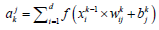
Where matrix x_i^k-1 is feature map of the k −1

Layer, a^j_k is a jth feature map of the kth layer, drepresents the number of input feature maps, w^k_ij is the weight parameter and b_j^k is the bias parameter which is randomly initialized.

f (x_i^k-1×w^k_ij+b_j^k) is the nonlinear activation function where we are utilizing the ReLU activation function in this research.

*Represents the convolution operation.

Pooling layer: It's commonly found immediately following the convolution layer. It's used to reduce the data's spatial dimension. A pooling operation reduces the network's parameters and prevents over fitting. The max-poling method is applied in this article.

Fully connected layer: The output value of each neuron in the connected layer is sent to the classifier after it interacts with all neurons in the preceding layer. The back-propagation algorithm is used to train all parameters in the neural network. The CNN methods reused in the classification of hyperspectral images are 2-Dimensional-Convilutional Neural Network and 3-Dimensional-Convilutional Neural Network. In this proposed method, we are using 3D-CNN with PCA, 3D-CNN without PCA, and comparing both of them.

3D-Convolution neural network

3D-Convolution: From hyperspectral images, 3D-convolution extracts spectral and spatial information. This can be computed by the below equation.

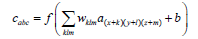
Where the c_abcis the output feature at the position (a,b,c), a_{(x+k)(y+l)(z+m)} represents input at the position (x+k, y+l, z+m) in which (k,l,m) denotes in its offset to (a, b, c) and w_klm weighted for the input. a_{(x+k)(y+l)(z+m)} with an offset of (k, l, m) in the convolution kernel the feature size is smaller.

ReLU activation: The Rectifier Linear Unit (ReLU) is a nonlinear function that operates in a nonlinear manner. If a neuron's input is positive, the ReLU accepts it; if the input is negative, it returns zero. The features of the ReLU activation function are rapid gradient progression, sparse activation, and minimal computing effort.

f (x) = max(0, x)

Where x is input data,

ReLU in 3D-CNN can improve the performance in the large majority of applications.

Proposed 3D-Convolution network model: Figure 11 shows the proposed 3D-CNN model for hyperspectral images. This model first uses the PCA for the reduction of data and then its reduced input to the proposed network model to extract features at different levels of layers, such as convolution layers, Max_pooling layers, and dense layers. Finally, classification is performed on fully connected layers and softmax functions. The number of fully connected layers and 3D convectional layers can be referred to in Tables 4 and 5 for two datasets [20].

Figure 11: Proposed 3D CNN model architecture for hyperspectral images.

Table 4: A brief summary of the proposed 3D-CNN model architecture for an Indian pines data set is provided in figure 6, with a 9 × 9 pixels window size for an Indian pines data set.

Table 5: A brief summary of the proposed 3D-CNN model architecture is shown in figure 6 with a 9 × 9 pixels window size.

Results and Discussion

To use the proposed 3D-CNN to classify different crops, 75% of each class's samples are selected as training samples, with the remaining samples being used as testing samples. All experiments were implemented by using Python 3 with Anaconda’s environment. To perform a fair comparison for all experiments with a learning rate of 0.001, an activation function Relu is used for all except the last layer with softmax, and patch sizes are set as 9 × 9 × 50 pixels and 11 × 11 × 50 pixels for the Indian pines dataset, and 9 × 9 × 10 pixels and 11 × 11 × 10 pixels for the ICRISAT data set, respectively. 50 and 10 are the bands selected by using the PCA method.

The confusion matrix was used to determine Average Accuracy (AA), Overall Accuracy (OA), and the Kappa coefficient (K) for evolution purposes. Figures 12 and 13 show the confusion matrix of both datasets [21].

Figure 12: Confusion matrix for Indian pines.

Figure 13: Confusion matrix for the ICRISAT dataset.

The average class-wise classification is presented by the Average Accuracy (AA), The number of correctly classified samples out of a total number of samples is calculated using the Overall Accuracy (OA). And finally, the kappa coefficient indicates a high level of agreement between the classification and ground truth maps. The statistical metric is called the kappa coefficient. F1-score, precision, and support all evolved into AA, OA, and Kappa. Figures 14 and 15 shows the convergence of accuracy and loss of our proposed 3D-CNN for 500 epochs with PCA of both datasets [22].

Figure 14: Accuracy and loss of the proposed 3D-CNN model for Indian pines data set.

Figure 15: Proposed 3D-CNN model’s accuracy and loss on the ICRISAT dataset.

The computational time is shown in Table 6, and the computational time depends on the available RAM [23].

Table 6: All experimental datasets have a compute time in minutes.

Tables 7 and 8 provide the detailed classification of each class in the two datasets with different window sizes and figures. Figure 16 shows the detailed class accuracy comparison between the Indian Pines dataset and the ICRISAT dataset [24].

Table 7: Detail accuracy of each class for Indian pines dataset.

Table 8: Detail accuracy of each class for ICRISAT dataset.

Figure 16: Comparison of detail class accuracy for Indian pine and ICRISAT datasets.

Figures 17 and 18 show the classification images and ground truth images with different window sizes of Indian pines dataset.

Figure 17: Classification image of the Indian Pines data set with window size: 9 × 9 and 11 × 11 pixels.

Figure 18: Ground truth image of the Indian pines data set with window size: 9 × 9 and 11 × 11 pixels.

Figures 19 and 20 are showing the classification images and ground truth images with different window sizes of ICRISAT dataset.

Figure 19: Classification image of the ICRISAT dataset with window size: 9 × 9 and 11 × 11 pixels.

Figure 20: Ground truth image of ICRISAT dataset with window size: 9 × 9 and 11 × 11 pixels.

Conclusion

The Deep Learning Method (DLM) for classifying crops using hyperspectral digital data was developed and validated in this work. It also used two datasets for the DLM and also used a customized 3D-CNN. 75% of samples in the Indian Pines dataset and 75% of samples in the ICRISAT dataset are selected as training samples, with the remaining 25% selected as testing samples for both datasets. The confusion matrix was used to calculate the average accuracy, overall accuracy, and kappa coefficient for the evolution. The customized 3D-CNN can notably improve over all classification accuracy on both datasets. The average accuracy, over all accuracy, and kappa coefficient of the Indian Pines dataset are 98.68%, 99.88%, and 99.86%. The average accuracy, over-all accuracy, and kappa coefficient of the ICRISAT dataset are 95.60%, 99.52%, and 98.23%. The computational times for all experiments in the Indian Pines dataset and the ICRISAT dataset are 0.6 minutes and 0.56 minutes, respectively. Furthermore, the DLM model of deep learning is used for crop health detection.

Author Contributions

Mr. S. Jamalaiah conducts the research and wrote the paper; Prof. K. Manjulavani guides the research; both authors had approved the final version.

References

1. Hong L, Zhang M. Object-oriented multiscale deep features for hyperspectral image classification. Int J Remote Sens. 2020; 41(14):5549-5572.

   [Crossref] [Google Scholar]

2. Bhosle K, Musande V. Evaluation of CNN model by comparing with convolutional autoencoder and deep neural network for crop classification on hyperspectral imagery. Geocarto Int. 2022; 37(3):813-827.

   [Crossref] [Google Scholar]

3. Bera S, Shrivastava VK. Analysis of various optimizers on deep convolutional neural network model in the application of hyperspectral remote sensing image classification. Int J Remote Sens. 2020; 41(7):2664-2683.

   [Crossref] [Google Scholar]

4. Mei S, Yuan X, Ji J, et al. Hyperspectral image spatial super-resolution via 3D full convolutional neural network. Remote Sens. 2017; 9(11):1139.

   [Crossref] [Google Scholar]

5. Srivastava V, Biswas B. Deep CNN feature fusion with manifold learning and regression for pixel classification in HSI images. J Exp Theor Artif Intell. 2020; 32(2):339-358.

   [Crossref] [Google Scholar]

6. Chen Y, Zhu K, Zhu L, et al. Automatic design of convolutional neural network for hyperspectral image classification. IEEE Trans Geosci Remote Sens. 2019; 57(9):7048-7066.

   [Crossref] [Google Scholar]

7. He M, Li B, Chen H. Multi-scale 3D deep convolutional neural network for hyperspectral image classification. In 2017 IEEE ICIP. 2017; 3904-3908. IEEE.

   [Crossref] [Google Scholar]

8. Yan Y, Ryu Y. Exploring Google Street View with deep learning for crop type mapping. ISPRS J Photogramm Remote Sens. 2021; 171:278-296.

   [Crossref] [Google Scholar]

9. Wang C, Ma N, Ming Y, et al. Classification of hyperspectral imagery with a 3D convolutional neural network and JM distance. Adv Space Res. 2019; 64(4):886-899.

   [Crossref] [Google Scholar]

10. Ahmadi SA, Mehrshad N. Spectral-spatial feature extraction method for hyperspectral images classification using multiscale superpixel and covariance map. Geocarto Int. 2022; 37(2):678-695.

    [Crossref] [Google Scholar]

11. Zhao X, Liang Y, Guo AJ, et al. Classification of small-scale hyperspectral images with multi-source deep transfer learning. Remote Sens Lett. 2020; 11(4):303-312.

    [Crossref] [Google Scholar]

12. Konduri VS, Kumar J, Hargrove WW, et al. Mapping crops within the growing season across the United States. Remote Sens Environ. 2020; 251:112048.

    [Crossref] [Google Scholar]

13. Zhong Y, Hu X, Luo C, et al. WHU-Hi: UAV-borne hyperspectral with high spatial resolution (H2) benchmark datasets and classifier for precise crop identification based on deep convolutional neural network with CRF. Remote Sens Environ. 2020; 250:112012.

    [Crossref] [Google Scholar]

14. Xu J, Zhu Y, Zhong R, et al. DeepCropMapping: A multi-temporal deep learning approach with improved spatial generalizability for dynamic corn and soybean mapping. Remote Sens Environ. 2020; 247:111946.

    [Crossref] [Google Scholar]

15. Zhao J, Zhong Y, Hu X, et al. A robust spectral-spatial approach to identifying heterogeneous crops using remote sensing imagery with high spectral and spatial resolutions. Remote Sens Environ. 2020; 239:111605.

    [Crossref] [Google Scholar]

16. Zhong L, Hu L, Zhou H. Deep learning based multi-temporal crop classification. Remote Sens Environ. 2019; 221:430-443.

    [Crossref] [Google Scholar]

17. Zhao H, Chen Z, Jiang H, et al. Evaluation of three deep learning models for early crop classification using sentinel-1A imagery time series—A case study in Zhanjiang, China. Remote Sens. 2019; 11(22):2673.

    [Crossref] [Google Scholar]

18. Ji S, Zhang C, Xu A, et al. 3D convolutional neural networks for crop classification with multi-temporal remote sensing images. Remote Sens. 2018; 10(1):75.

    [Crossref] [Google Scholar]

19. Ge Z, Cao G, Li X, et al. Hyperspectral image classification method based on 2D–3D CNN and multibranch feature fusion. IEEE J Sel Top Appl Earth Obs Remote Sens. 2020; 13:5776-5788.

    [Crossref] [Google Scholar]

20. Zhang C, Atkinson PM, George C, et al. Identifying and mapping individual plants in a highly diverse high-elevation ecosystem using UAV imagery and deep learning. ISPRS J Photogramm Remote Sens. 2020; 169:280-291.

    [Crossref] [Google Scholar]

21. Kanthi M, Sarma TH, Bindu CS. A 3D-deep CNN based feature extraction and hyperspectral image classification. In2020 IEEE India Geosci Remote Sens Symposium (InGARSS) 2020; 229-232.

    [Crossref] [Google Scholar]

22. Hu W, Huang Y, Wei L, et al. Deep convolutional neural networks for hyperspectral image classification. J Sens. 2015; 1-2.

    [Crossref] [Google Scholar]

23. Xu Z, Guan K, Casler N, et al. A 3D convolutional neural network method for land cover classification using LiDAR and multi-temporal Landsat imagery. ISPRS J Photogramm Remote Sens. 2018; 144:423-434.

    [Crossref] [Google Scholar]

24. Fallah-Adl H, JaJa J, Liang S, et al. Efficient algorithms for atmospheric correction of remotely sensed data. In Proceedings of the 1995 ACM/IEEE conference on Supercomputing 1995.

    [Crossref] [Google Scholar]